METHODS FOR PERFORMANCE EVALUATION OF SINGLE AXIS POSITIONING SYSTEMS: DYNAMIC STRAIGHTNESS
R. Fesperman, B. O'Connor, and J. Ellis
INTRODUCTION
Many new ultra-precision linear positioning systems are finding their way into emerging technologies that are requiring exceptional straightness performance during both static/quasi-static and dynamic positioning conditions. A few examples of these technologies include photovoltaic panel scribing, wafer dicing, and laser machining. Measuring and specifying static/quasi-static straightness is a well-defined process described in existing performance standards [1, 2]. A dynamic straightness test for identifying the amplitude of vibration during the acceleration and deceleration of machine tool axes is provided by ISO 230-8 [3]. However, a standard test method for characterizing and specifying dynamic straightness for single axis linear positioning systems does not currently exist. As a result, many manufacturers and users of linear positioning systems have developed their own internal methods and standards, which have led to customer confusion and ambiguity.
To help mitigate confusion, members from industry, academia, and government are working to develop a new positioning performance standard [4] that includes a new test method for characterizing straightness of a linear positioning system under dynamic conditions. In this paper, we discuss a test method for characterizing dynamic straightness. Descriptions of measurement setups, measurement and analysis procedures, and suggestions for reporting dynamic straightness results are presented.
STRAIGHTNESS
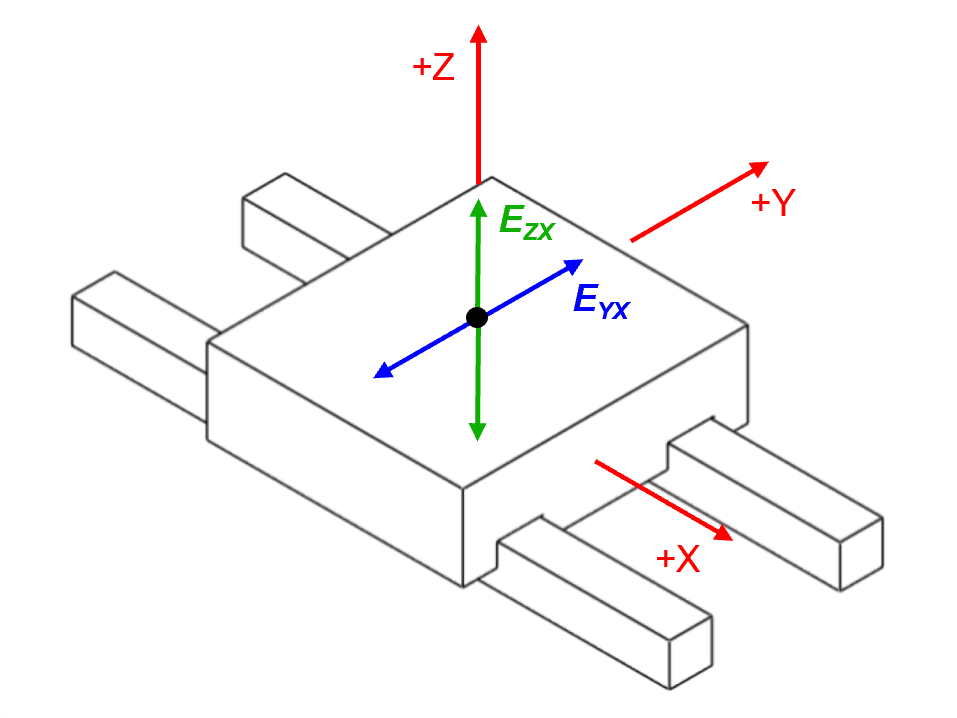
Straightness of a linear positioning system is characterized by measuring the motions of the carriage in the two directions orthogonal to the nominal direction of motion, see Figure 1. Under static and quasi-static conditions, the straightness errors are nominally the result of the geometric errors of the positioning system components. During dynamic conditions, straightness errors can be additionally affected by the forces and moments inherent in the dynamic system, e.g., drive forces occurring during acceleration and deceleration [3, 5]. As a result, straightness errors can change during static to dynamic transitions.
Applications in which linear positioning systems are used vary widely and the acceleration and deceleration regions differ for each. This diversity creates a challenge for specifying dynamic straightness. In some applications, such as constant velocity scanning (CVS), the process (e.g., manufacturing or measurement) may only occur during the constant velocity region of the velocity profile and therefore may not be affected by the acceleration and deceleration regions. Characterizing straightness over the acceleration and deceleration regions may be impractical when specifying and/or selecting positioning systems for CVS applications. However, other applications that include motions such as raster scanning and circular contouring, are affected by the acceleration and deceleration regions. Including these regions in the characterization and specification of dynamic straightness may be beneficial for these and similar applications. For these reasons, it may be important to consider the velocity profile for a given dynamic condition when characterizing and specifying dynamic straightness.
VELOCITY PROFILES
Velocity (or motion) profiles used for driving positioning systems can vary in form. Profiles can range from the most common and simplest profiles such as triangular or trapezoidal to more complex profiles that control the level of jerk (e.g., S-curve). Each profile differs by the method used to transition (e.g., time rate of change) from one commanded velocity to another. The smoothness of the transitions can affect straightness by introducing unwanted forces and moments on the moving element of the positioning system. Accurate characterization and a detailed understanding of dynamic straightness performance may be enhanced by the identification of the transitions regions. Identifying the transition regions requires detailed information about the velocity profile and its parameters (e.g., drive forces, accelerations and time constants). Most modern controllers allow access and exporting of profile data. Alternatively, the profile data can be Velocity (or motion) profiles used for driving positioning systems can vary in form. Profiles can range from the most common and simplest profiles such as triangular or trapezoidal to more complex profiles that control the level of jerk (e.g., S-curve). Each profile differs by the method used to transition (e.g., time rate of change) from one commanded velocity to another. The smoothness of the transitions can affect straightness by introducing unwanted forces and moments on the moving element of the positioning system. Accurate characterization and a detailed understanding of dynamic straightness performance may be enhanced by the identification of the transitions regions. Identifying the transition regions requires detailed information about the velocity profile and its parameters (e.g., drive forces, accelerations and time constants). Most modern controllers allow access and exporting of profile data. Alternatively, the profile data can be provided by the manufacturer or it can be determined by characterizing the positioning system following standard test methods such as the Feedrate and Acceleration method described in ASME B5.54 [1]. Similar test methods are being considered for inclusion in the new standard.
STRAIGHTNESS MEASUREMENT
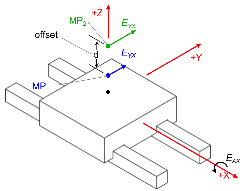
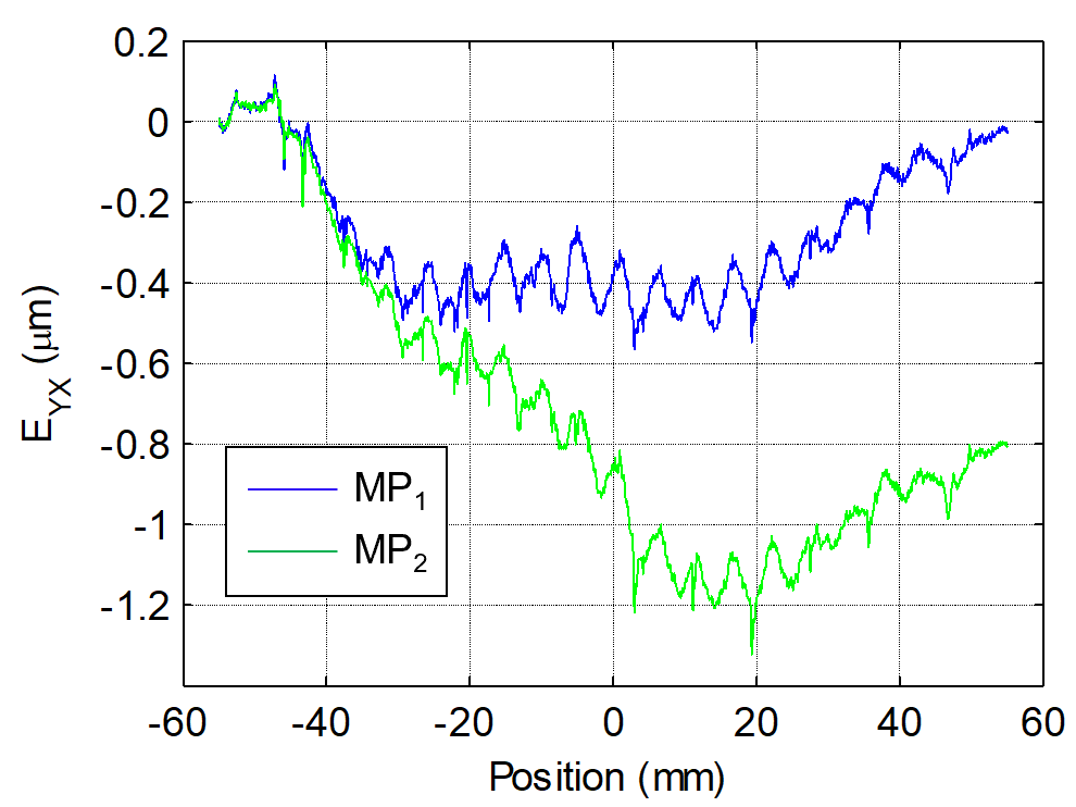
Normally, straightness errors are characterized by measuring the trajectory of a point that is rigidly attached to the moving element (e.g., carriage) of a linear positioning system. Furthermore, straightness errors (i.e., straightness measurement results) are also affected by the angular motions/errors of the positioning system and thus have different magnitudes along different point trajectories, as shown in Figure 2. The differences in magnitude are related by the offset distance between points (Abbe' Offset) and the angular motions of the positioning system. This concept is known as the Bryan Principle [6].
Theoretically, the measured point can be located anywhere around the positioning system. Because the magnitude changes with point location, it is recommended that the location of the measured point correspond to the location of the functional point [2], i.e., the point where work for the intended application is occurring. However, spatial constraints may limit the ability to measure straightness errors at the functional point. For this reason it is recommended that the measured point be located as close to the functional point as possible, with the point’s location with respect to the axis coordinate frame being well documented [4] and measurements made of the relevant angular errors. Resulting measurement data should then be transformed to represent the straightness errors at the functional point of the intended application.
Representing the straightness of a single axis positioning system as the measured motion of a point rigidly attached to the moving element (i.e., constant with respect to the axis coordinate frame) may be beneficial for the user when comparing positioning systems. Such available data can be employed by the user to simulate the straightness performance for different applications having different functional points.
General Measurement Setup
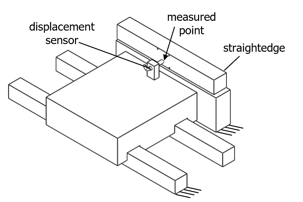
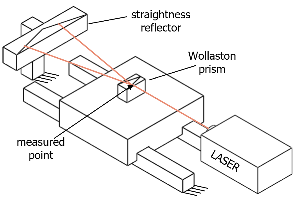
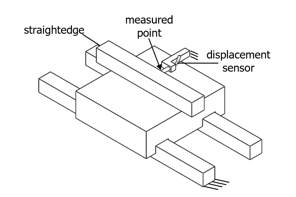
The two most common methods for measuring straightness include measurement of a straightness reference (straightedge) by a displacement sensor (e.g., capacitance sensor) and use of a laser straightness interferometer consisting of a Wollaston prism and a straightness reflector. The equipment and method chosen should reflect the expected performance of the positioning system and the results of a test uncertainty evaluation [7]. Reversal procedures can be used to further limit the uncertainties due to straightedge errors. With either method, straightness can be determined by measuring with a fixed or moving sensor setup (Figures 3 and 4). Ideally, the setup chosen should reflect how the positioning system is used in the final application.
Moving Sensor Setup
In moving sensor setups (Figure 3), the displacement sensor or prism is attached to the traversing element of the positioning system (e.g., carriage) and measures with respect to a stationary straightedge or straightness reflector fixed to the base of the positioning system. With these types of measurements, the location of the sensor (i.e., sensing surface) or prism represents the location of the measured point. Throughout the measurement, the location of the measured point with respect to the axis coordinate frame is constant and the resulting measurement data represents the straightness of the point’s trajectory. It should be noted that displacement sensors with sensor cables attached may experience false readings due to cable movements. Cable management should be considered or a fixed sensor setup eliminating cable movements may be used.
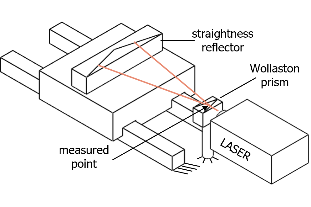
Fixed Sensor Setup
In fixed sensor setups (Figure 4), the displacement sensor or prism is held stationary (fixed to the base of the positioning system) and measures against a traversing straightedge or reference reflector attached to the moving element of the positioning system. With this type of measurement setup, the location of the measured point with respect to the axis coordinate frame is not constant and varies as a function of axis position. If the user wishes to represent the measured data as the straightness of a single measurement point (i.e., identical to the moving sensor measurement), then a transformation must be performed on the data. A transformation, in turn, requires an additional measurement of the appropriate angular positioning errors.
With either measurement setup, the straightedge should be aligned to the axis motion within an appropriate level of alignment uncertainty and should be supported to minimize deformations along the functional surface.
Dynamic Considerations
Because accelerations and decelerations (i.e., drive forces) can affect the dynamic straightness error, the velocity and acceleration regions of the positioning profile should be identified. These regions may be identified by recording the position of the axis encoders during the straightness measurement, directly measuring the position of the axis or measured point with an external sensor, or performing a separate velocity and acceleration measurement for the programmed motion profile. In addition to drive forces, straightness errors may also be affected by gravity or the mass of the payload that the positioning system is intended to carry. For these reasons, the positioning profile, payload mass, and center of payload mass that best represents the intended use of the positioning system should be considered and applied during dynamic straightness measurements.
System Condition
Prior to commencing measurements, the positioning system should be exercised to thermally stabilize the system. At minimum, axis warm-up should include five back-and-forth movements between the first and last target points. The velocity/motion profile and payload employed should be the same profile and payload used for the straightness measurement. If deemed necessary, controller tuning in response to the measurement payload should be considered acceptable as long as the payload is closely related to the payload of the application.
Dynamic Straightness Test Procedure
The test should be conducted at a programmed feedrate and load that best replicates the conditions of the application in which the positioning system is intended to be used. If the positioning system is to be used as a general purpose system or a predefined programmed velocity is not available, then three different tests should be conducted at 10%, 50%, and 100% of the maximum programmable feedrate (velocity). The default traverse distance should consume the maximum allowable distance for the positioning system. A trigger or digital marker should be used to initiate or mark the measurement at the beginning of both positive and negative directions of motion. Any dwells added to the motion profile should be documented.
Procedure
1) Align the measuring equipment with the trajectory of the measurement point under evaluation. 2) Exercise the positioning system following the recommendations described in System Condition. 3) Program the positioning system to continuously move the carriage with the predetermined velocity profile. 4) Set the data acquisition system sampling rate to accurately capture and detect the acceleration and deceleration regions. 5) Document all test parameters. 6) Perform five sets of bidirectional or unidirectional measurements. Record time, axis position, and the corresponding raw displacement readings for straightness.
Dynamic Straightness Analysis
Measurement data should be processed using software. Post-process filtering should be performed on raw measurement data and the type of filter (e.g., low-pass 4th-order Butterworth filter) and cutoff frequency should be reported. All transformations should be performed before straightness calculations.
Full Travel Straightness Analysis
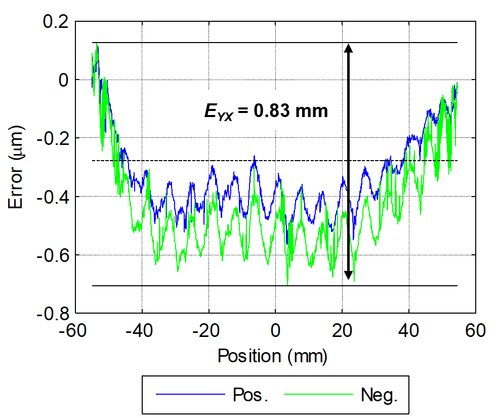
Full travel straightness can be reported as either bidirectional or unidirectional. For each set of measurements, the best-fit line corresponding to the raw or filtered data is calculated using the least-squares method over the full positioning range of the stage. For bidirectional measurements, the best fit line is calculated for either the positive or negative direction of travel, but not both. The minimum distance between two lines enveloping the straightness data (unidirectional or bidirectional) and parallel to the least-squares best-fit line is the straightness value for the measurement and filter condition. See Figure 5. The averages of the five straightness values and the expanded measurement uncertainty are reported as the full travel straightness error of the axis for the specified velocity profile and filter condition.
Constant Velocity Straightness Analysis
Constant velocity straightness can be reported as either bidirectional or unidirectional. For each set of measurements, the best-fit line corresponding to the raw or filtered constant velocity data is calculated using the least-squares method. For bidirectional measurements the best fit line is calculated for either the positive or negative direction of travel, but not both. The minimum distance between two lines enveloping the constant velocity straightness data (unidirectional or bidirectional) and parallel to the least-squares best-fit line is the straightness value for the measurement and filter condition. The average of five straightness values and the expanded measurement uncertainty are reported as the constant velocity straightness.
Reporting and Presentation of Results
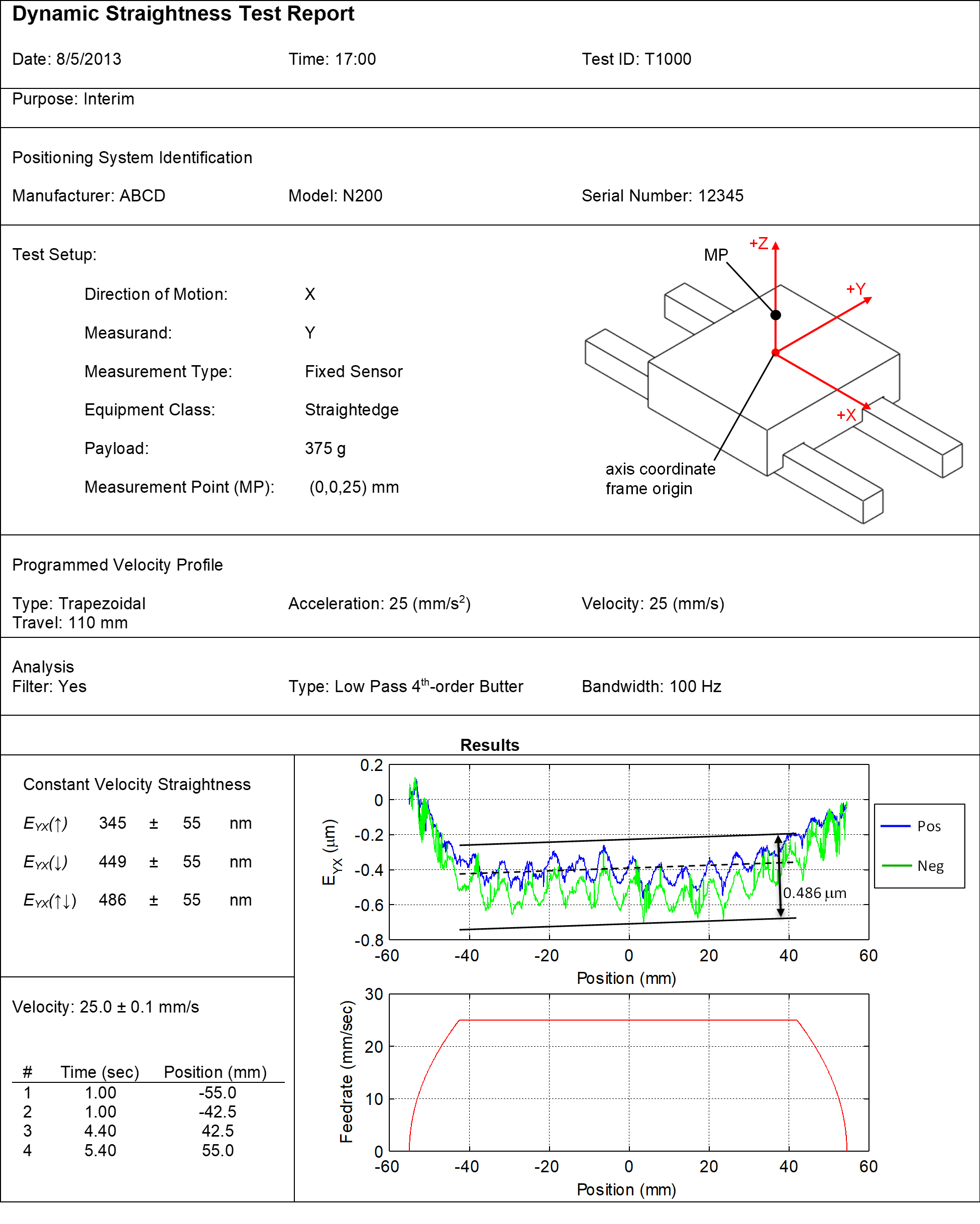
Dynamic straightness of a positioning system should be identified as either the straightness of full travel for a defined motion/velocity profile or the straightness over a constant velocity region. For either case, a velocity profile plot identifying the acceleration regions should be provided along with a plot of dynamic straightness. In addition, settling times and regions for constant velocity measurements should be identified. A dynamic straightness plot should contain the average of the five measurement runs and the two parallel lines that envelope the straightness data. The straightness values, the filter parameters, the load, and location of the measured point should be reported. An example of a dynamic straightness report for constant velocity straightness is provided as Figure 6.
COMMENTS
A new standard test method for characterizing and specifying the dynamic straightness of linear positioning systems was presented. The work is ongoing and the robustness of the method is being evaluated by characterizing the dynamic straightness for a variety of single axis positioning systems.
REFERENCES
- ASME B5.54-2005, Methods for Performance Evaluation of Computer Numerically Controlled Machining Centers, 2005.
- ISO 230-1:2012, Test code for machine tools – Part 1: Geometric accuracy of machines operating under no-load or finishing conditions, 2012.
- ISO/TR 230-8, Test code for machine tools – Part 8: Vibrations, Technical Report, 2010.
- Fesperman R, Brown N, Elliott K, Ellis J, Grabowski A, Ludwick S, Maneuf S, O’Connor B, Woody S, Methods for Performance Evaluation of Single Axis Positioning Systems: A New Standard, Proceedings of the ASPE Annual Meeting, 2013.
- Miller J, Hocken R, Ramanan V, Feng Q, Foundation for Dynamic Metrology of Machine Tools, Proceedings of the ASPE Annual Meeting, 1999.
- Bryan J, The Abbe’ Principle Revisited: An Updated Interpretation, Precision Engineering, 1979.
- ISO/TR 230-9:2005E, Test code for machine tools – Part 9: Estimation of measurement uncertainty for machine tool tests according to series ISO 230, basic equations, 2005.
* No approval or endorsement of any commercial product by the National Institute of Standards and Technology is intended or implied. Certain commercial equipment, instruments, or materials are identified in this report in order to facilitate understanding. Such identification does not imply recommendation or endorsement by the National Institute of Standards and Technology, nor does it imply that the materials or equipment identified are necessarily the best available for the purpose. This publication was prepared by United States Government employees as part of their official duties and is, therefore, a work of the U.S. Government and not subject to copyright.